Deflection of a simply supported beam under uniform load

Introduction

This study deals with the deflec­tion of a sim­ply sup­ported beam of span $L$ car­ry­ing a uni­formly dis­trib­uted load $q$. The aim is to com­pare the closed ana­lyt­i­cal solu­tion with a numer­i­cal solu­tion obtained by the finite-dif­fer­ence method¹ and to show under which con­di­tions the Bernoulli–Navier hypoth­e­sis is suf­fi­cient. Back in the 1960s such val­ues were read from tables; today a script of a few dozen lines does the job.

The max­i­mum deflec­tion at midspan is given by

$$w_{\max} = \frac{5\,q\,L^4}{384\,E\,I},$$

where $E$ is Young’s mod­u­lus and $I$ the sec­ond moment of area. For steel, $E = 210\,\mathrm{GPa}$; tim­ber is roughly ten times softer. Codes usu­ally limit the rel­a­tive deflec­tion $w_{\max}/L$ to 1/250.

The for­mula rests on the Bernoulli–Navier hypoth­e­sis, which neglects the shear con­tri­bu­tion to deflec­tion. What gov­erns its mag­ni­tude is not slen­der­ness as such but the ratio of bend­ing to shear stiff­ness: for a uni­form load,

$$\frac{w_{\mathrm{V}}}{w_{\mathrm{M}}} = \frac{q L^2 / (8\,G\,A_{\mathrm{s}})} {5\,q\,L^4 / (384\,E\,I)} = 9.6\,\frac{E\,I}{G\,A_{\mathrm{s}}\,L^2},$$

where $G$ is the shear mod­u­lus and $A_{\mathrm{s}}$ the shear area. Only for a homo­ge­neous rec­tan­gu­lar sec­tion does this reduce to $\approx 2.5\,(h/L)^2$, so that for $h/L = 1/20$ the shear part is about 0.6 %—which is where the pop­u­lar slen­der­ness rule of thumb comes from. For sand­wich, thin-walled or com­pos­ite sec­tions with a low $G\,A_{\mathrm{s}}$, shear may mat­ter even for a very slen­der beam and Tim­o­shenko the­ory is appro­pri­ate.

Input data and parametric study

The fol­low­ing table sum­marises a para­met­ric study of 36 com­bi­na­tions of span and load. The table delib­er­ately runs over one page to exer­cise the repeated table header in print.

Results for spans above 8.0 m clearly vio­late the 1/250 limit and call for a deeper sec­tion or a cam­ber.

Computational script

The ana­lyt­i­cal solu­tion is ver­i­fied by the fol­low­ing script. The lines are delib­er­ately long to exer­cise code wrap­ping in print.

"""Simply supported beam deflection: analytical vs. numerical (finite differences)."""
import numpy as np

def analytical_solution(L: float, q: float, E: float, I: float, n: int = 101) -> np.ndarray:
    """Return the deflection curve w(x) = q x (L^3 - 2 L x^2 + x^3) / (24 E I)."""
    x = np.linspace(0.0, L, n)
    return q * x * (L**3 - 2.0 * L * x**2 + x**3) / (24.0 * E * I)

def numerical_solution(L: float, q: float, E: float, I: float, n: int = 101) -> np.ndarray:
    """Solve E I w'''' = q by finite differences with w(0) = w(L) = 0, w''(0) = w''(L) = 0."""
    h = L / (n - 1)
    A = np.zeros((n, n)); b = np.full(n, q * h**4 / (E * I))
    for i in range(2, n - 2):
        A[i, i-2:i+3] = [1.0, -4.0, 6.0, -4.0, 1.0]
    A[0, 0] = A[n-1, n-1] = 1.0; b[0] = b[n-1] = 0.0          # w = 0 at supports
    A[1, 0:3] = [1.0, -2.0, 1.0]; b[1] = 0.0                   # w'' = 0 (left hinge)
    A[n-2, n-3:n] = [1.0, -2.0, 1.0]; b[n-2] = 0.0             # w'' = 0 (right hinge)
    return np.linalg.solve(A, b)

if __name__ == "__main__":
    L, q, E, I = 6.0, 10_000.0, 210e9, 83.3e-6
    w_a = analytical_solution(L, q, E, I)
    w_n = numerical_solution(L, q, E, I)
    print(f"analytical w_max = {1000 * w_a.max():.3f} mm, numerical w_max = {1000 * w_n.max():.3f} mm")
    print(f"relative deviation = {abs(w_n.max() - w_a.max()) / w_a.max():.2e}")

Graphical results

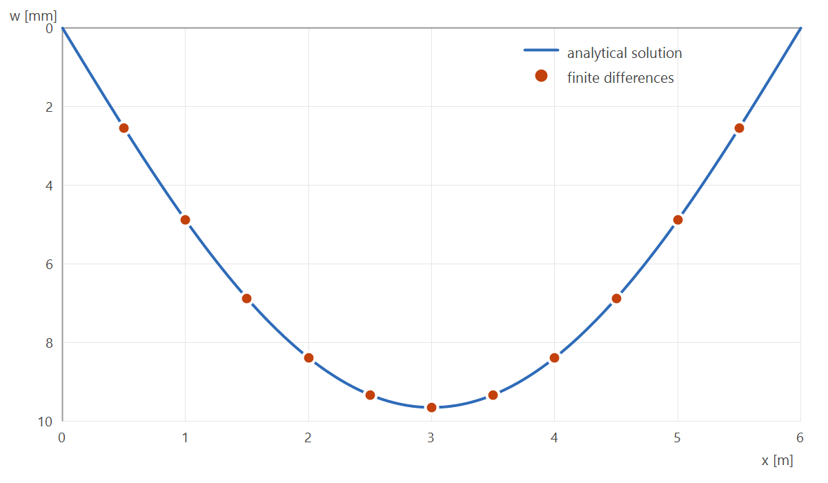
The deflec­tion curves of both solu­tions are plot­ted in the fol­low­ing fig­ure.

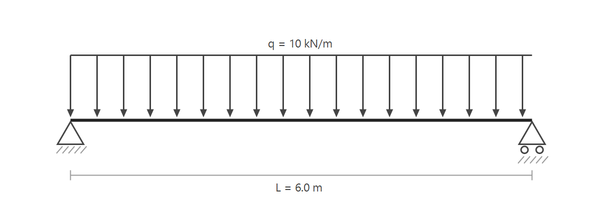
The sta­tic scheme, stored under the same file name in a dif­fer­ent folder:

Source vs. result

This doc­u­ment was pro­duced from plain Mark­down. The block below is the lit­eral source text (typo­graphic rules are delib­er­ately not applied inside code blocks):

She said "the span is 6 m" - and she's right: pages 10-20 of the report
list a 40x60 mm section tested at 25 °C... Don't forget section 3.

And this is how mdprint type­sets the very same text:

She said “the span is 6 m”—and she’s right: pages 10–20 of the report list a 40×60 mm sec­tion tested at 25 °C… Don’t for­get sec­tion 3.

The dif­fer­ence lives in the details that decide leg­i­bil­ity: curly quotes, an em dash, an en dash in the range, a real mul­ti­pli­ca­tion sign, a proper apos­tro­phe and a bound num­ber–unit pair. Math is type­set; code and paths stay untouched.

Conclusion

The numer­i­cal solu­tion dif­fers from the ana­lyt­i­cal one by less than 0.01 %, con­firm­ing both approaches. The inline rela­tion $w(x) = \frac{q x (L^3 - 2Lx^2 + x^3)}{24 E I}$ can there­fore be used for quick checks². A def­i­n­i­tion to close with:

Ser­vice­abil­ity limit state

A state beyond which the struc­ture no longer meets its oper­a­tional require­ments, although no fail­ure occurs.